AT 309 Week 15 - Final Data Product

Introduction

              This serves as the culmination of our progress throughout AT 309, both figuratively and literally. In this report, I have used all of the skills I have learned throughout this semester to interpret and make professional maps from all of the data we have collected over the semester. The area of focus for this report is the Purdue Turf Farm (PTF), one of our major UAS mission areas. Over the semester, we have collected data from this area using a variety of platforms and sensors. For this project, we are using the data from 6 different mapping missions.

First, in week 3, we used the Skydio 2+ to collect data from this area. Then, in week 5, we used the Mavic 2 Pro. Finally, in Week 7, we used the M300 with 4 different sensors: the Sony A7 RGB camera, the Zenmuse P1 RGB camera, the Zenmuse H20T thermal camera, and the Micasense RedEdge hyperspectral camera. From this, I made 3 different maps for each mission: an orthomosaic, a Digital Surface Model (DSM), and a shaded DSM, for a total of 18 maps. A digital surface model maps the elevation of a surface and includes any objects that might be in the area, like trees, buildings, and cars. The data products are sorted by platform, as I have included some details about the processing for each one. This helps keep the data products in their each section, and we can see the differences in the outputs between each platform.

Results

Skydio 2+

Purdue Turf Farm – Week 3

Deliverables:

-          Orthomosaic (Figure 1)

-          Digital Surface Model (Figure 2)

-          Shaded Digital Surface Model (Figure 3)

Mission Date: 9/6/2024Altitude: 60 mPlatform: Skydio 2+

Projection	Cell Size (cm)	Min Elevation (m)	Max Elevation (m)
WGS 1984 UTM Zone 16N - Transverse Mercator	X = 2.963 Y = 2.963	195.656	221.647

Figure 1: Skydio Ortho with Flight Lines

Figure 2: Skydio DSM

Figure 3: Skydio Shaded DSM

Figure 4: "Adjust Images" Settings for Skydio

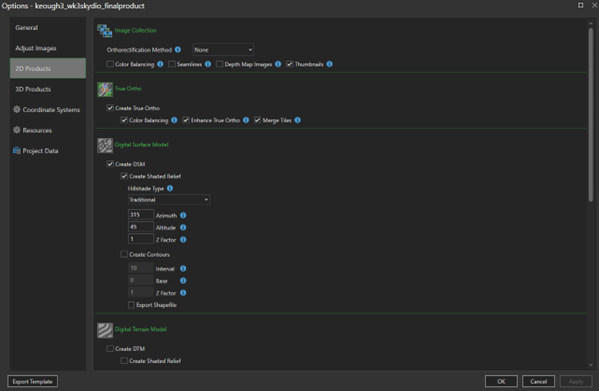
Figure 5: "2D Products" Settings for Skydio

Figure 6: Coordinate System Information for Skydio

Mavic 2 Pro

Purdue Turf Farm – Week 5

Deliverables:

-          Orthomosaic (Figure 7)

-          Digital Surface Model (Figure 8)

-          Shaded Digital Surface Model (Figure 9)

Mission Date: 9/6/2024Altitude: 60 mPlatform: Mavic 2 Pro

Projection	Cell Size (cm)	Min Elevation (m)	Max Elevation (m)
WGS 1984 UTM Zone 16N - Transverse Mercator	X = 1.450 Y = 1.450	210.145	236.150

Figure 7: Mavic Ortho with Flight Lines

Figure 8: Mavic DSM

Figure 9: Mavic Shaded DSM

Figure 10: "Adjust Images" Setting for Mavic

Figure 11: "2D Products" Setting for Mavic

Figure 12: Coordinate System Information for Mavic

M300 (Sony A7 PPK)

Purdue Turf Farm – Week 7

Deliverables:

-          Orthomosaic (Figure 13Figure 7)

-          Digital Surface Model (Figure 14Figure 8)

-          Shaded Digital Surface Model (Figure 15Figure 9)

Mission Date: 10/4/2024Altitude: 60 mPlatform: M300Sensor: Sony A7

Projection	Cell Size (cm)	Min Elevation (m)	Max Elevation (m)
WGS 1984 UTM Zone 16N - Transverse Mercator	X = 0.647 Y = 0.647	210.242	229.757

Figure 13: M300 w/ Sony A7 Orthomosaic

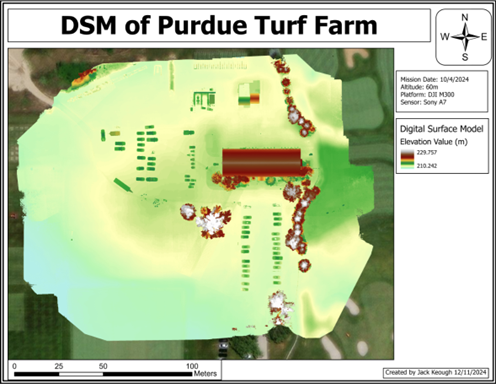
Figure 14: M300 w/ Sony A7 DSM

Figure 15: M300 w/ Sony A7 Shaded DSM

Figure 16: "Adjust Images" Setting for A7 Mission

Figure 17: "2D Products" Settings for A7 Mission

Figure 18: Coordinate System Information for A7 Mission

M300 (P1 RTK)

Purdue Turf Farm – Week 7

Deliverables:

-          Orthomosaic (Figure 19Figure 7)

-          Digital Surface Model (Figure 20Figure 8)

-          Shaded Digital Surface Model (Figure 21Figure 9)

Mission Date: 10/4/2024Altitude: 60 mPlatform: M300Sensor: Zenmuse P1 RTK

Projection	Cell Size (cm)	Min Elevation (m)	Max Elevation (m)
WGS 1984 UTM Zone 16N – Transverse Mercator	X = 0.755 Y = 0.755	211.661	237.525

Figure 19: M300 w/ P1 Ortho

Figure 20: M300 w/ P1 DSM

Figure 21: M300 w/ P1 Shaded DSM

Figure 22: "Adjust Images" Settings for P1 Mission

Figure 23: "2D Products" Settings for P1 Mission

Figure 24: Coordinate System Information for P1 Mission

M300 (H20T Thermal)

Purdue Turf Farm – Week 7

Deliverables:

-          Orthomosaic (Figure 25Figure 7)

-          Digital Surface Model (Figure 26Figure 8)

-          Shaded Digital Surface Model (Figure 27Figure 9)

Mission Date: 10/4/2024Altitude: 60 mPlatform: M300Sensor: Zenmuse H20T Thermal

Projection	Cell Size (cm)	Min Elevation (m)	Max Elevation (m)
WGS 1984 UTM Zone 16N - Transverse Mercator	X = 6.619 Y = 6.619	239.618	245.970

Figure 25: M300 w/ H20T Ortho

Figure 26: M300 w/ H20T DSM

Figure 27: M300 w/ H20T Shaded DSM

Figure 28: "Adjust Images" Settings for H20T Thermal Mission

Figure 29: "2D Products" Settings for  H20T Thermal Mission

Figure 30: Coordinate System Information for H20T Thermal Mission

M300 (Micasense RedEdge)

Purdue Turf Farm – Week 7

Deliverables:

-          Orthomosaic (Figure 31Figure 7)

-          Digital Surface Model (Figure 32Figure 8)

-          Shaded Digital Surface Model (Figure 33Figure 9)

Mission Date: 10/4/2024Altitude: 60 mPlatform: M300Sensor: Micasense RedEdge

Projection	Cell Size (cm)	Min Elevation (m)	Max Elevation (m)
WGS 1984 UTM Zone 16N - Transverse Mercator	X = 4.245 Y= 4.245	210.092	228.283

Figure 31: M300 w/ RedEdge Ortho

Figure 32: M300 w/ RedEdge DSM

Figure 33: M300 w/ RedEdge Shaded DSM

Figure 34: "Adjust Images" Settings for RedEdge Mission

Figure 35: "2D Products" Settings for RedEdge Mission

Figure 36: Coordinate System Information for RedEdge Mission

Conclusion

              This ended up being a lot of pages, but I was very happy to find that I’ve become quite efficient with ArcGIS Pro and Drone2Map. I was able to make the maps very quickly, although I had to go back a couple times to fix any mistakes I made, which mostly consisted of forgetting to remove the service credits. One timesaver for me was the ability to save layout templates. This made the process of making clean, consistent maps a breeze and probably saved me hours of formatting. I was able to pull processed data for some of the missions from previous labs, but I still had to do quite a bit of processing myself. All of the processing seemed to go well except for the H20T, which came out looking poor. I’m not sure where I went wrong with that, but it was still good enough to generate decent looking maps. Perhaps it’s a lesson, and the point is to show that a thermal camera is not the best tool to go about making orthomosaics and DSMs. As for the conclusions from the data itself? Regarding the turf farm, I think we have learned that it has a building, some trees, and maybe a couple of cars parked there at any moment. The thing that is really of note comes down to the differences between the sensors. Some created better products than others, however most of them would suffice for a surface level analysis like this. When scaled up, I think all the sensors would hold their own, apart from the H20T (at least the way I processed it). Overall, I think the work we did as a class this semester as well as the bits of research into ArcGIS Pro on my own helped me get this done with a level of quality that I can be proud of, although I may look back to this next year and be disgusted with my work. I doubt it would be that severe, and for now I think my products came out great.